Overview
We will explore the ProtConn indicator which was developed to report international conservation targets (Saura et al. 2017), the indicator offers you an analysis of protected areas connectivity for a particular region.
ProtConn estimation for a single ecoregion
In the following example, we will estimate the ProtConn indicator and fractions in one ecoregion using two dispersal distances (10 and 30 km) and a connection probability of 0.5. Also, we will use a Transboundary buffer of 50 km (50000 meters) from the edge of the region (transboundary_type = “region”, ?MK_ProtConn), the distance between protected areas will be using centroids.
region <- regions[1,]
test.1 <- MK_ProtConn(nodes = Protected_areas, region = region,
                      area_unit = "ha", distance = list(type= "centroid"),
                      distance_thresholds = c(10000, 30000), probability = 0.5,
                      transboundary = 50000, transboundary_type = "region",
                      LA = NULL, plot = TRUE, write = NULL,
                      intern = FALSE)
Exploring the results for a single ecoregion
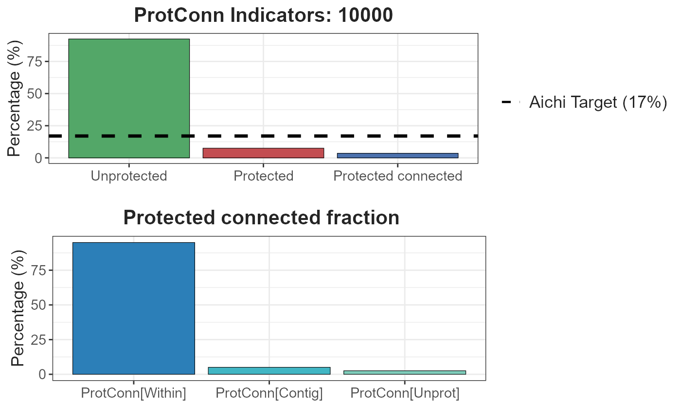
- Result 10 km:
test.1$d10000$`Protected Connected (Viewer Panel)`
| Index | Value | ProtConn indicator | Percentage |
|---|---|---|---|
| EC(PC) | 130282.77 | Prot | 7.5228 |
| PC | 1.2000e-03 | Unprotected | 92.4772 |
| Maximum landscape attribute | 3708497.35 | ProtConn | 3.5131 |
| Protected surface | 278983.74 | ProtUnconn | 4.0097 |
| RelConn | 46.6991 | ||
| ProtConn_Prot | 97.4444 | ||
| ProtConn_Trans | 0.0000 | ||
| ProtConn_Unprot | 2.5556 | ||
| ProtConn_Within | 94.9554 | ||
| ProtConn_Contig | 5.0446 | ||
| ProtConn_Within_land | 3.3359 | ||
| ProtConn_Contig_land | 0.1772 | ||
| ProtConn_Unprot_land | 0.0898 | ||
| ProtConn_Trans_land | 0.0000 |
test.1$d10000
#> $`Protected Connected (Viewer Panel)`
#>
#> $`ProtConn Plot`
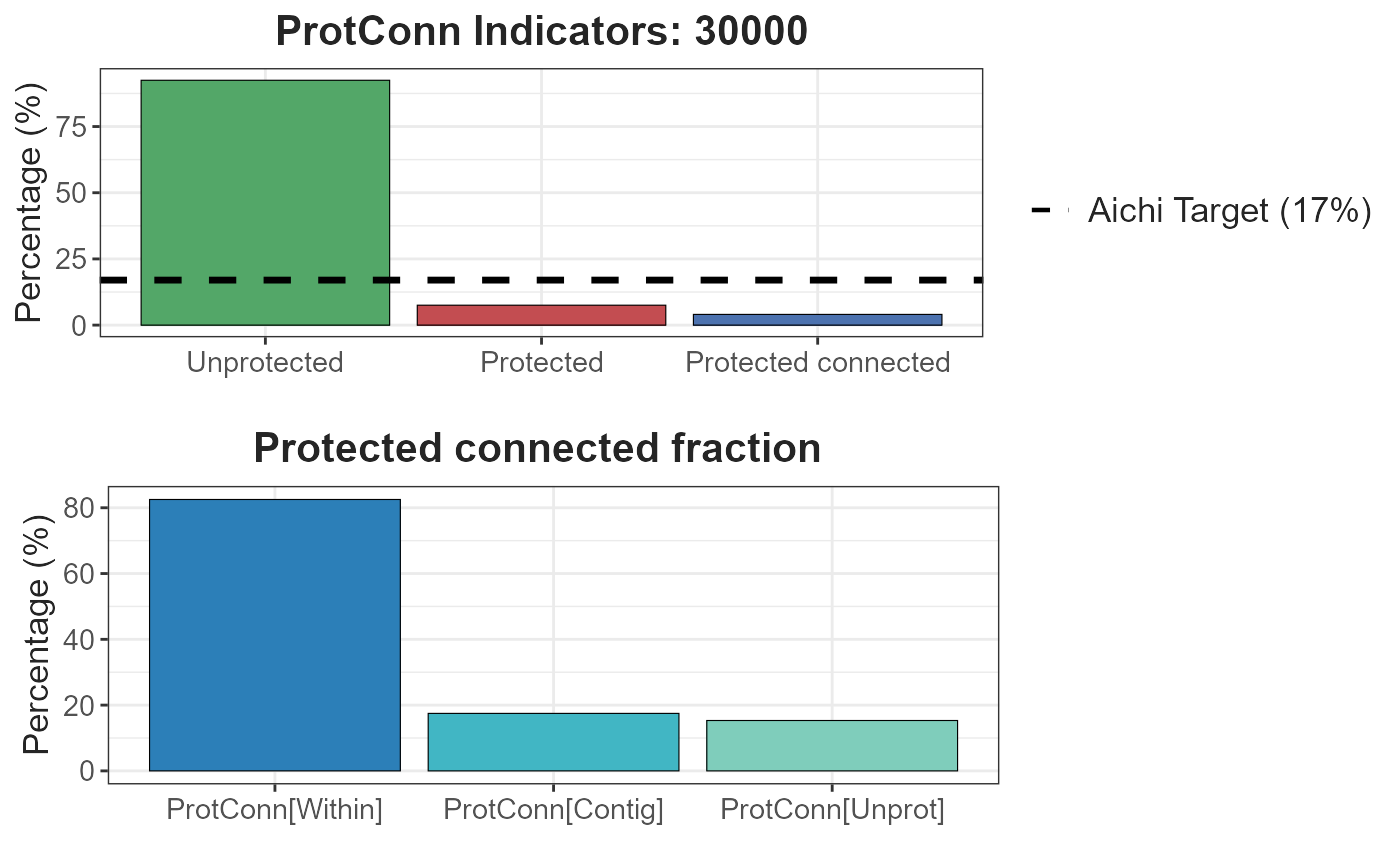
- Result 30 km:
test.1$d30000$`Protected Connected (Viewer Panel)`
| Index | Value | ProtConn indicator | Percentage |
|---|---|---|---|
| EC(PC) | 149921.76 | Prot | 7.5228 |
| PC | 1.6000e-03 | Unprotected | 92.4772 |
| Maximum landscape attribute | 3708497.35 | ProtConn | 4.0427 |
| Protected surface | 278983.74 | ProtUnconn | 3.4802 |
| RelConn | 53.7385 | ||
| ProtConn_Prot | 84.6797 | ||
| ProtConn_Trans | 0.0000 | ||
| ProtConn_Unprot | 15.3203 | ||
| ProtConn_Within | 82.5167 | ||
| ProtConn_Contig | 17.4833 | ||
| ProtConn_Within_land | 3.3359 | ||
| ProtConn_Contig_land | 0.7068 | ||
| ProtConn_Unprot_land | 0.6193 | ||
| ProtConn_Trans_land | 0.0000 |
test.1$d30000
#> $`Protected Connected (Viewer Panel)`
#>
#> $`ProtConn Plot`
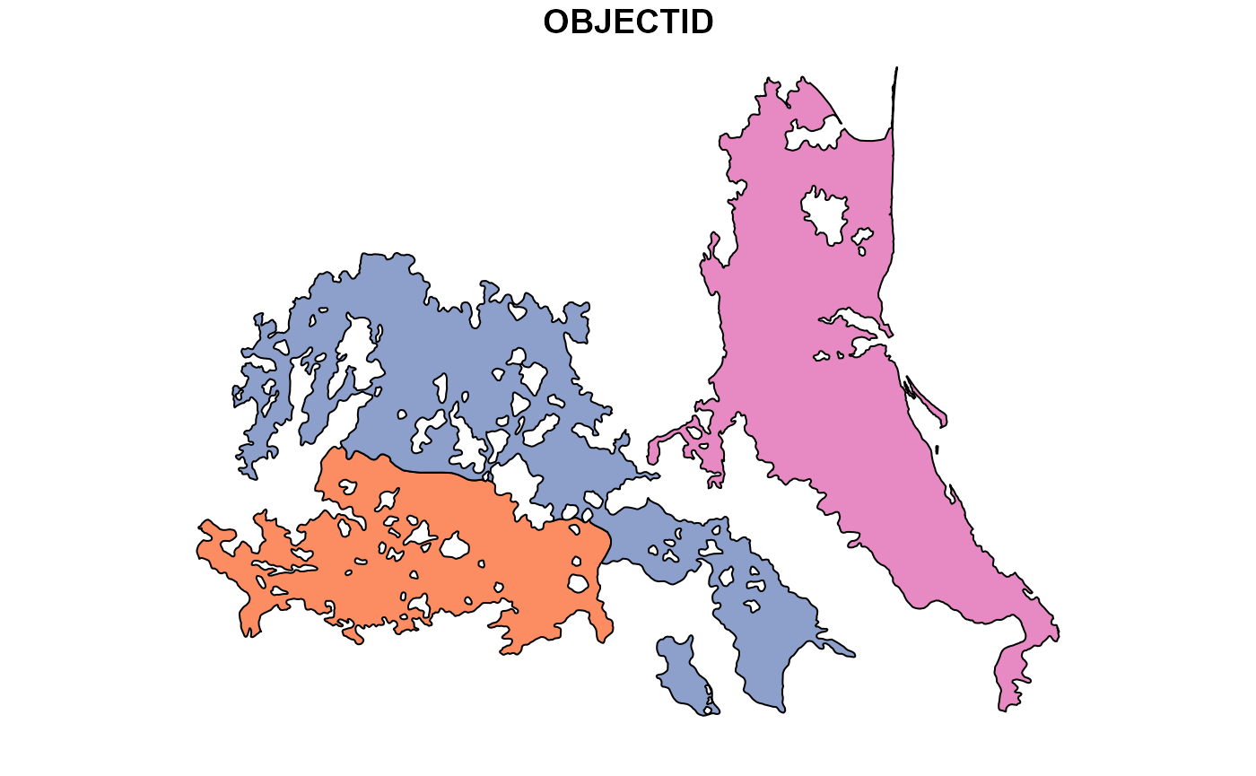
ProtConn estimation for two or more ecoregions.
Now, we will use the three ecoregions. The processing time will be longer when using more regions, although we can reduce it using the parallel argument.
test.2 <- MK_ProtConnMult(nodes = Protected_areas, regions = regions,
                          area_unit = "ha", distance = list(type= "centroid"),
                          distance_thresholds = c(10000, 30000), probability = 0.5,
                          transboundary = 50000, transboundary_type = "region",
                          plot = FALSE, write = NULL,
                          parallel = NULL, intern = FALSE)
Exploring some results
- Table summary result:
names(test.2)
#> [1] "ProtConn_10000" "ProtConn_30000"
test.2$ProtConn_10000$ProtConn_overall10000
| ProtConn indicator | Values (%) | SD | SEM | normal.lower | normal.upper | basic.lower | basic.upper | percent.lower | percent.upper | bca.lower | bca.upper | |
|---|---|---|---|---|---|---|---|---|---|---|---|---|
| 3 | Prot | 6.916 | 1.332 | 0.769 | 5.669 | 8.103 | 5.996 | 8.443 | 5.390 | 7.837 | 5.390 | 7.732 |
| 4 | Unprotected | 93.084 | 1.332 | 0.769 | 91.897 | 94.331 | 91.557 | 94.004 | 92.163 | 94.610 | 92.163 | 93.899 |
| 5 | ProtConn | 2.894 | 1.050 | 0.606 | 1.903 | 3.824 | 2.274 | 4.106 | 1.682 | 3.513 | 1.682 | 3.495 |
| 6 | ProtUnconn | 4.023 | 0.321 | 0.186 | 3.728 | 4.316 | 3.695 | 4.337 | 3.708 | 4.351 | 3.708 | 4.237 |
| 7 | RelConn | 40.796 | 8.383 | 4.840 | 32.835 | 48.193 | 34.893 | 50.391 | 31.200 | 46.699 | 31.200 | 45.225 |
| 8 | ProtConn_Prot | 97.302 | 2.105 | 1.215 | 95.365 | 99.213 | 95.272 | 99.475 | 95.130 | 99.333 | 95.130 | 98.703 |
| 9 | ProtConn_Trans | 0.000 | 0.000 | 0.000 | 0.000 | 0.000 | 0.000 | 0.000 | 0.000 | 0.000 | 0.000 | 0.000 |
| 10 | ProtConn_Unprot | 2.698 | 2.105 | 1.215 | 0.787 | 4.635 | 0.525 | 4.728 | 0.667 | 4.870 | 0.667 | 4.098 |
| 11 | ProtConn_Within | 88.251 | 5.841 | 3.372 | 82.524 | 93.393 | 81.547 | 92.239 | 84.263 | 94.955 | 84.263 | 91.815 |
| 12 | ProtConn_Contig | 11.749 | 5.841 | 3.372 | 6.607 | 17.476 | 7.761 | 18.453 | 5.045 | 15.737 | 5.045 | 15.313 |
| 13 | ProtConn_Within_land | 2.571 | 1.001 | 0.578 | 1.617 | 3.452 | 1.805 | 3.703 | 1.438 | 3.336 | 1.438 | 3.071 |
| 14 | ProtConn_Contig_land | 0.323 | 0.198 | 0.114 | 0.146 | 0.512 | 0.097 | 0.469 | 0.177 | 0.549 | 0.177 | 0.549 |
| 15 | ProtConn_Unprot_land | 0.065 | 0.036 | 0.021 | 0.030 | 0.098 | 0.040 | 0.107 | 0.023 | 0.090 | 0.023 | 0.087 |
| 16 | ProtConn_Trans_land | 0.000 | 0.000 | 0.000 | 0.000 | 0.000 | 0.000 | 0.000 | 0.000 | 0.000 | 0.000 | 0.000 |
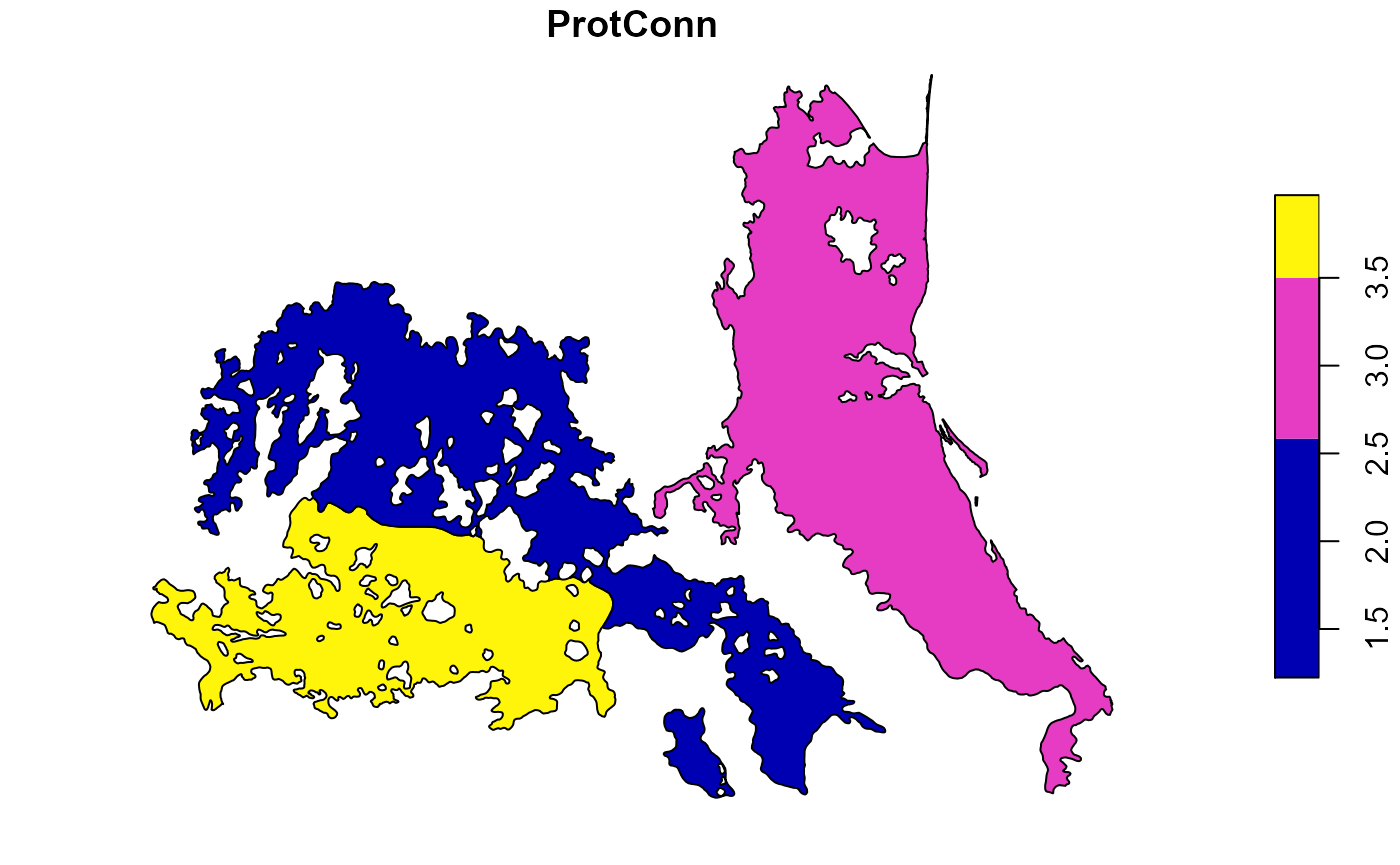
- Shapefile result:
test.2$ProtConn_10000$ProtConn_10000
#> Simple feature collection with 3 features and 17 fields
#> Geometry type: GEOMETRY
#> Dimension:     XY
#> Bounding box:  xmin: 2287307 ymin: 792114.5 xmax: 3085667 ymax: 1392441
#> CRS:           BOUNDCRS[
#>     SOURCECRS[
#>         PROJCRS["unknown",
#>             BASEGEOGCRS["unknown",
#>                 DATUM["World Geodetic System 1984",
#>                     ELLIPSOID["WGS 84",6378137,298.257223563,
#>                         LENGTHUNIT["metre",1]],
#>                     ID["EPSG",6326]],
#>                 PRIMEM["Greenwich",0,
#>                     ANGLEUNIT["degree",0.0174532925199433],
#>                     ID["EPSG",8901]]],
#>             CONVERSION["unknown",
#>                 METHOD["Lambert Conic Conformal (2SP)",
#>                     ID["EPSG",9802]],
#>                 PARAMETER["Latitude of false origin",12,
#>                     ANGLEUNIT["degree",0.0174532925199433],
#>                     ID["EPSG",8821]],
#>                 PARAMETER["Longitude of false origin",-102,
#>                     ANGLEUNIT["degree",0.0174532925199433],
#>                     ID["EPSG",8822]],
#>                 PARAMETER["Latitude of 1st standard parallel",17.5,
#>                     ANGLEUNIT["degree",0.0174532925199433],
#>                     ID["EPSG",8823]],
#>                 PARAMETER["Latitude of 2nd standard parallel",29.5,
#>                     ANGLEUNIT["degree",0.0174532925199433],
#>                     ID["EPSG",8824]],
#>                 PARAMETER["Easting at false origin",2500000,
#>                     LENGTHUNIT["metre",1],
#>                     ID["EPSG",8826]],
#>                 PARAMETER["Northing at false origin",0,
#>                     LENGTHUNIT["metre",1],
#>                     ID["EPSG",8827]]],
#>             CS[Cartesian,2],
#>                 AXIS["(E)",east,
#>                     ORDER[1],
#>                     LENGTHUNIT["metre",1,
#>                         ID["EPSG",9001]]],
#>                 AXIS["(N)",north,
#>                     ORDER[2],
#>                     LENGTHUNIT["metre",1,
#>                         ID["EPSG",9001]]]]],
#>     TARGETCRS[
#>         GEOGCRS["WGS 84",
#>             DATUM["World Geodetic System 1984",
#>                 ELLIPSOID["WGS 84",6378137,298.257223563,
#>                     LENGTHUNIT["metre",1]]],
#>             PRIMEM["Greenwich",0,
#>                 ANGLEUNIT["degree",0.0174532925199433]],
#>             CS[ellipsoidal,2],
#>                 AXIS["geodetic latitude (Lat)",north,
#>                     ORDER[1],
#>                     ANGLEUNIT["degree",0.0174532925199433]],
#>                 AXIS["geodetic longitude (Lon)",east,
#>                     ORDER[2],
#>                     ANGLEUNIT["degree",0.0174532925199433]],
#>             ID["EPSG",4326]]],
#>     ABRIDGEDTRANSFORMATION["Transformation from unknown to WGS84",
#>         METHOD["Geocentric translations (geog2D domain)",
#>             ID["EPSG",9603]],
#>         PARAMETER["X-axis translation",0,
#>             ID["EPSG",8605]],
#>         PARAMETER["Y-axis translation",0,
#>             ID["EPSG",8606]],
#>         PARAMETER["Z-axis translation",0,
#>             ID["EPSG",8607]]]]
#>   OBJECTID    EC(PC)     PC   Prot Unprotected ProtConn ProtUnconn RelConn
#> 1       61 130282.77 0.0012 7.5228     92.4772   3.5131     4.0097 46.6991
#> 2      143  98619.63 0.0003 5.3895     94.6105   1.6815     3.7080 31.2002
#> 3      772 238055.88 0.0012 7.8370     92.1630   3.4865     4.3505 44.4882
#>   ProtConn_Prot ProtConn_Trans ProtConn_Unprot ProtConn_Within ProtConn_Contig
#> 1       97.4444              0          2.5556         94.9554          5.0446
#> 2       95.1302              0          4.8698         85.5352         14.4648
#> 3       99.3326              0          0.6674         84.2633         15.7367
#>   ProtConn_Within_land ProtConn_Contig_land ProtConn_Unprot_land
#> 1               3.3359               0.1772               0.0898
#> 2               1.4383               0.2432               0.0819
#> 3               2.9379               0.5487               0.0233
#>   ProtConn_Trans_land                       geometry
#> 1                   0 POLYGON ((2553705 1009434, ...
#> 2                   0 MULTIPOLYGON (((2475555 121...
#> 3                   0 MULTIPOLYGON (((2933834 137...
- It is important not to forget that you can change the type of distance using the distance (
see, distancefile()) argument:
Euclidean distances: * distance = list(type= “centroid”) * distance = list(type= “edge”)
Least cost distances, you need a raster with resistance values, it is recommended that the range of values be from 1 to 10: * distance = list(type= “least-cost”, resistance = “resistance raster”) * distance = list(type= “commute-time”, resistance = “resistance raster”)
Reference:
- Saura, S., Bastin, L., Battistella, L., Mandrici, A., & Dubois, G. (2017). Protected areas in the world’s ecoregions: How well connected are they? Ecological Indicators, 76, 144–158.